Linkage Synthesis
This tutorial covers classical mechanism synthesis methods for designing four-bar linkages that achieve specific motion requirements. Instead of optimizing an existing linkage, synthesis methods compute linkage dimensions directly from your specifications.
Overview
Pylinkage implements three classical synthesis approaches:
Function Generation: Design a linkage where input crank angle maps to a specific output rocker angle relationship.
Path Generation: Design a linkage where a coupler point traces through specified precision points.
Motion Generation: Design a linkage where a coupler body passes through specified poses (position + orientation).
All methods are based on Burmester theory and Freudenstein’s equation, classical results from kinematic synthesis.
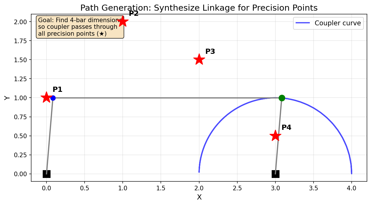
Path generation: find a four-bar linkage whose coupler passes through specified precision points (red stars).
Quick Start: Path Generation
The most common use case is designing a linkage where the coupler traces a specific path:
from pylinkage.synthesis import path_generation
import pylinkage as pl

# Define points the coupler should pass through
precision_points = [
    (0.0, 1.0),
    (1.0, 2.0),
    (2.0, 1.5),
    (3.0, 0.5),
]

# Find linkages that achieve this path
result = path_generation(precision_points)

print(f"Found {len(result)} candidate solutions")

# Visualize the first solution
if result.solutions:
    linkage = result.solutions[0]
    pl.show_linkage(linkage)
Expected output:
Found 4 candidate solutions
The synthesis returns multiple candidate linkages because the mathematical problem typically has several solutions.
Function Generation
Function generation designs a linkage where the input crank angle maps to a specific output rocker angle. This is useful for mechanisms that need to transform rotational motion with a specific ratio.
Theory: Freudenstein’s Equation
For a four-bar linkage with links of lengths \(L_1\) (crank), \(L_2\) (coupler), \(L_3\) (rocker), and \(L_4\) (ground), Freudenstein’s equation relates input angle \(\phi\) to output angle \(\psi\):
where:
Given 3 input/output angle pairs, we can solve for \(K_1, K_2, K_3\) and thus determine the link ratios.
Example: Three Precision Points
import math
from pylinkage.synthesis import function_generation
import pylinkage as pl

# Define input/output angle pairs (phi, psi) in radians
angle_pairs = [
    (0.0, 0.0),                    # Position 1
    (math.pi / 6, math.pi / 4),    # Position 2: 30° -> 45°
    (math.pi / 3, math.pi / 2),    # Position 3: 60° -> 90°
]

# Synthesize the linkage
result = function_generation(angle_pairs)

if result:
    print(f"Found {len(result)} solutions")
    for i, sol in enumerate(result.raw_solutions):
        print(f"\nSolution {i + 1}:")
        print(f"  Crank length (L1):   {sol.crank_length:.4f}")
        print(f"  Coupler length (L2): {sol.coupler_length:.4f}")
        print(f"  Rocker length (L3):  {sol.rocker_length:.4f}")
        print(f"  Ground length (L4):  {sol.ground_length:.4f}")

    # Visualize the first solution
    linkage = result.solutions[0]
    pl.show_linkage(linkage)
else:
    print("No valid solutions found")
    for warning in result.warnings:
        print(f"Warning: {warning}")
Expected output:
Found 1 solutions

Solution 1:
  Crank length (L1):   1.0000
  Coupler length (L2): 2.4142
  Rocker length (L3):  1.7321
  Ground length (L4):  2.0000
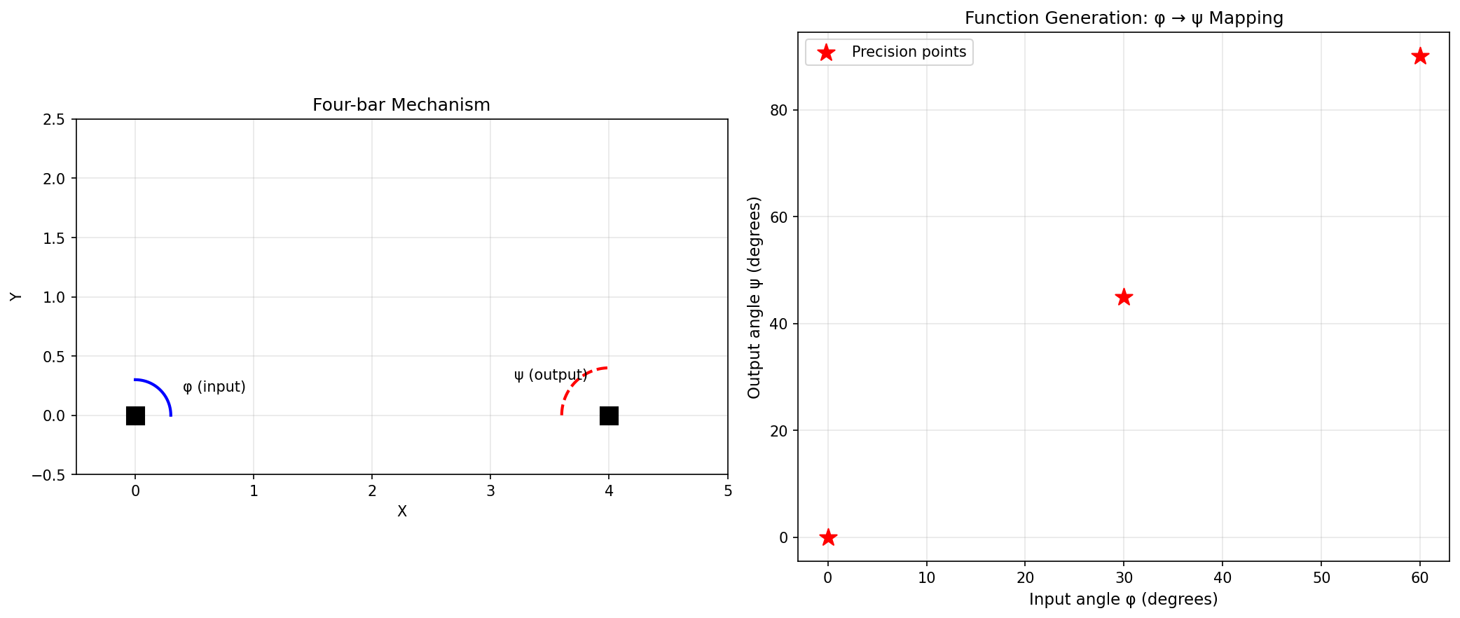
Function generation: the left plot shows the mechanism at different input angles, the right plot shows the input-output angle relationship.
Verifying Function Generation
You can verify that the synthesized linkage achieves the desired angle mapping:
from pylinkage.synthesis import verify_function_generation

# Check if synthesized linkage achieves the angle pairs
errors = verify_function_generation(linkage, angle_pairs)

print("Verification results:")
for i, (phi, psi, error) in enumerate(zip(
    [p[0] for p in angle_pairs],
    [p[1] for p in angle_pairs],
    errors
)):
    print(f"  Point {i+1}: phi={math.degrees(phi):.1f}°, "
          f"psi={math.degrees(psi):.1f}°, error={error:.6f}")
Path Generation
Path generation finds linkages where a coupler point traces through specified positions. Unlike function generation, the coupler orientation at each point is not specified, making this problem more complex.
Theory: Burmester Curves
Burmester theory identifies all possible fixed pivot locations (center points) and moving pivot locations (circle points) such that the moving pivot traces circular arcs through the precision positions. By selecting compatible pairs of dyads (ground-coupler connections), we can construct four-bar linkages.
Basic Path Generation
from pylinkage.synthesis import path_generation
import pylinkage as pl

# Four precision points define the path
points = [
    (0.0, 0.0),
    (2.0, 1.0),
    (4.0, 0.5),
    (5.0, -1.0),
]

result = path_generation(points)

print(f"Found {len(result)} solutions")
print(f"Warnings: {result.warnings}")

# Examine each solution
for i, linkage in enumerate(result.solutions):
    print(f"\nSolution {i + 1}:")
    # Show the linkage dimensions
    constraints = list(linkage.get_num_constraints())
    print(f"  Constraints: {constraints}")

    # Verify the path
    loci = list(linkage.step())
    coupler_path = [step[-1] for step in loci]
    print(f"  Path traces {len(coupler_path)} points")
Example result (may vary):
Found 3 solutions
Warnings: []

Solution 1:
  Constraints: [0.314, 1.5, 2.8, 1.2]
  Path traces 20 points
Path Generation with Timing
Sometimes you need the coupler to reach each point at a specific crank angle.
Use path_generation_with_timing:
import math
from pylinkage.synthesis import path_generation_with_timing, PrecisionPoint

# Define points with associated crank angles
precision_points = [
    PrecisionPoint(x=0.0, y=0.0, theta=0.0),
    PrecisionPoint(x=2.0, y=1.0, theta=math.pi / 2),
    PrecisionPoint(x=4.0, y=0.5, theta=math.pi),
    PrecisionPoint(x=5.0, y=-1.0, theta=3 * math.pi / 2),
]

result = path_generation_with_timing(precision_points)

if result:
    print(f"Found {len(result)} timed solutions")
Motion Generation
Motion generation is the most constrained synthesis type: the coupler body must pass through specified poses (position AND orientation).
Theory
For motion generation, we specify poses \((x, y, \theta)\) where \(\theta\) is the coupler orientation. Burmester theory then finds attachment points on the coupler that trace circular arcs compatible with fixed pivots on the ground.
Three-Pose Synthesis
With exactly 3 poses, the solution is typically unique (or a small set):
from pylinkage.synthesis import motion_generation, Pose
import pylinkage as pl

# Define poses: (x, y, orientation_angle)
poses = [
    Pose(x=0.0, y=0.0, theta=0.0),
    Pose(x=2.0, y=1.0, theta=0.3),
    Pose(x=3.0, y=0.5, theta=0.6),
]

result = motion_generation(poses)

print(f"Found {len(result)} solutions")

if result:
    linkage = result.solutions[0]
    print("\nLinkage configuration:")
    for joint in linkage.joints:
        print(f"  {joint.name}: ({joint.x:.2f}, {joint.y:.2f})")

    pl.show_linkage(linkage)
Expected output:
Found 2 solutions

Linkage configuration:
  Crank: (0.00, 1.00)
  Output: (2.50, 0.75)
Four-Pose and Five-Pose Synthesis
With more poses, the problem becomes over-constrained, requiring least-squares or iterative methods:
from pylinkage.synthesis import motion_generation_3_poses, Pose

# For 4+ poses, use the iterative solver
poses = [
    Pose(0.0, 0.0, 0.0),
    Pose(1.0, 0.5, 0.2),
    Pose(2.0, 0.8, 0.4),
    Pose(3.0, 0.6, 0.6),
]

# motion_generation handles this internally
result = motion_generation(poses)

if result:
    print(f"Found {len(result)} approximate solutions")
    # Solutions may not pass exactly through all poses
Working with Synthesis Results
All synthesis functions return a SynthesisResult object:
from pylinkage.synthesis import path_generation

result = path_generation(points)

# Check if solutions were found
if result:
    print("Solutions found!")

# Number of solutions
print(f"Count: {len(result)}")

# Iterate over linkages
for linkage in result:
    print(linkage.name)

# Access the underlying solutions with full parameters
for sol in result.raw_solutions:
    print(f"Crank: {sol.crank_length}")
    print(f"Coupler: {sol.coupler_length}")
    print(f"Rocker: {sol.rocker_length}")
    print(f"Ground: {sol.ground_length}")

# Check for warnings
for warning in result.warnings:
    print(f"Warning: {warning}")
Creating Linkages from Dimensions
If you already know the link lengths, create a four-bar directly:
from pylinkage.synthesis import fourbar_from_lengths
import pylinkage as pl

linkage = fourbar_from_lengths(
    crank_length=1.0,
    coupler_length=3.0,
    rocker_length=3.0,
    ground_length=4.0,
)

# Check Grashof condition
from pylinkage.synthesis import grashof_check, is_crank_rocker

grashof = grashof_check(1.0, 3.0, 3.0, 4.0)
print(f"Grashof type: {grashof}")

if is_crank_rocker(1.0, 3.0, 3.0, 4.0):
    print("This is a crank-rocker mechanism")

pl.show_linkage(linkage)
Expected output:
Grashof type: GrashofType.CRANK_ROCKER
This is a crank-rocker mechanism
Grashof Analysis
The Grashof criterion determines the type of motion a four-bar can achieve:
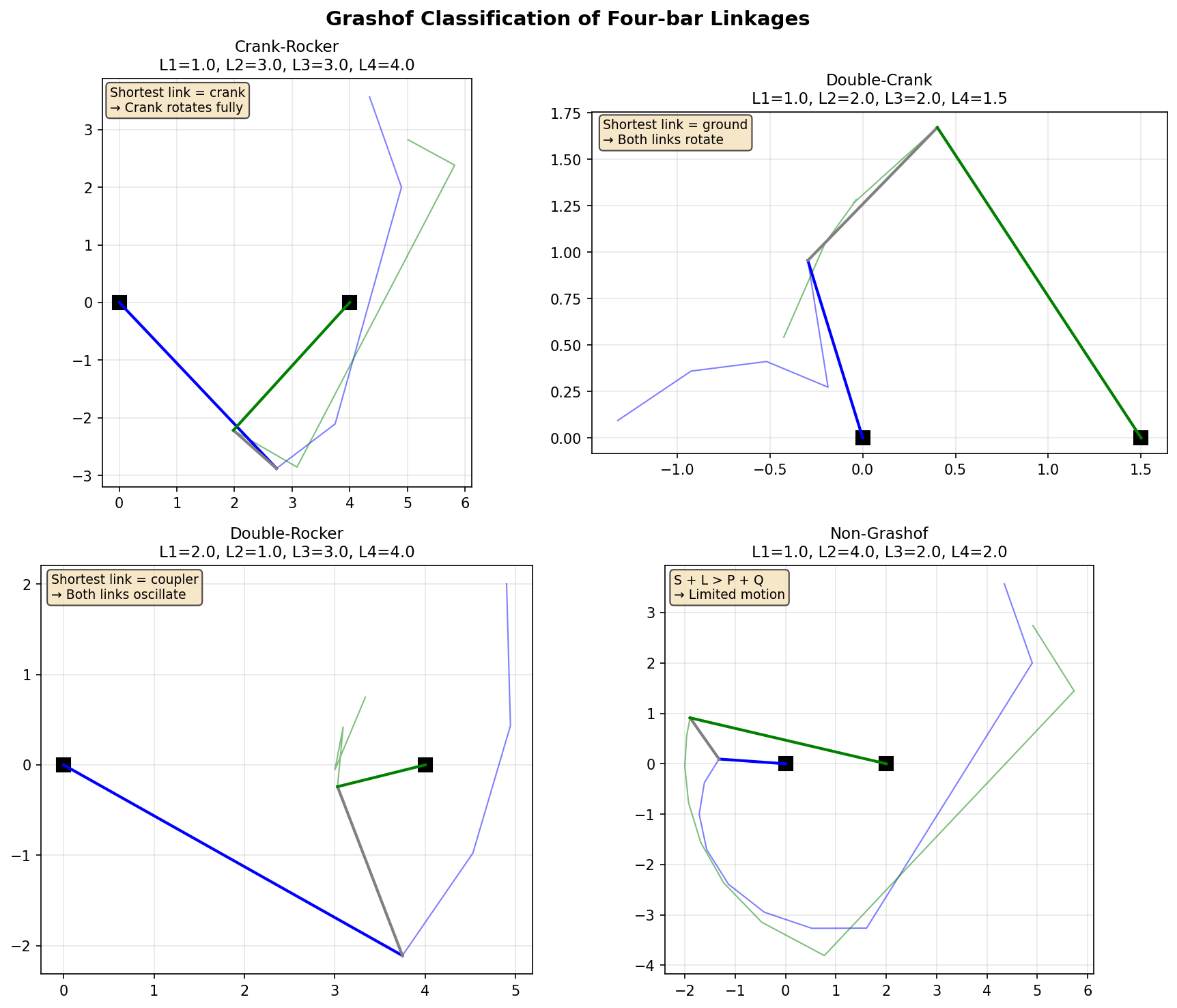
The four types of four-bar linkages based on the Grashof criterion: crank-rocker, double-crank, double-rocker, and non-Grashof.
from pylinkage.synthesis import grashof_check, GrashofType, is_grashof

# Link lengths: crank, coupler, rocker, ground
L1, L2, L3, L4 = 1.0, 3.0, 3.0, 4.0

# Check if Grashof (shortest + longest <= sum of other two)
print(f"Is Grashof: {is_grashof(L1, L2, L3, L4)}")

# Get specific type
grashof_type = grashof_check(L1, L2, L3, L4)

if grashof_type == GrashofType.CRANK_ROCKER:
    print("Crank makes full rotations, rocker oscillates")
elif grashof_type == GrashofType.DOUBLE_CRANK:
    print("Both crank and rocker make full rotations")
elif grashof_type == GrashofType.DOUBLE_ROCKER:
    print("Both crank and rocker oscillate")
elif grashof_type == GrashofType.CHANGE_POINT:
    print("Change-point mechanism (special case)")
else:
    print("Non-Grashof: no link can rotate fully")
Advanced: Burmester Curve Analysis
For research or advanced applications, access the underlying Burmester computations:
from pylinkage.synthesis import (
    compute_all_poles,
    compute_circle_point_curve,
    select_compatible_dyads,
    Pose,
)

poses = [
    Pose(0, 0, 0),
    Pose(1, 1, 0.5),
    Pose(2, 0.5, 1.0),
]

# Compute relative rotation poles between poses
poles = compute_all_poles(poses)
print(f"Poles: {poles}")

# Compute the circle-point curve (locus of valid attachment points)
curve = compute_circle_point_curve(poses)

# Select compatible dyad pairs to form a complete 4-bar
dyads = select_compatible_dyads(curve, poses)
print(f"Found {len(dyads)} compatible dyad pairs")
Synthesis vs Optimization
When to use synthesis:
You have specific precision requirements (exact points/angles to hit)
You want mathematically optimal solutions (not approximations)
The problem fits the classical synthesis framework (3-5 positions)
When to use optimization (PSO):
You have a complex objective function (not just precision points)
You need to optimize for velocity, acceleration, or other properties
The problem doesn’t fit classical synthesis patterns
You want to explore a wide design space
You can also combine both approaches: use synthesis to get a good starting point, then use PSO to fine-tune for additional objectives.
from pylinkage.synthesis import path_generation
import pylinkage as pl

# Step 1: Synthesize initial design
points = [(0, 0), (1, 1), (2, 0.5), (3, -0.5)]
result = path_generation(points)

if result:
    linkage = result.solutions[0]

    # Step 2: Fine-tune with PSO for additional objectives
    @pl.kinematic_minimization
    def combined_fitness(loci, **kwargs):
        # Precision point error
        output_path = [step[-1] for step in loci]
        point_error = sum(
            min((p[0]-t[0])**2 + (p[1]-t[1])**2 for p in output_path)
            for t in points
        )

        # Additional: minimize mechanism size
        all_points = [p for step in loci for p in step]
        bbox = pl.bounding_box(all_points)
        size = (bbox[1] - bbox[3]) * (bbox[2] - bbox[0])

        return point_error + 0.1 * size

    bounds = pl.generate_bounds(linkage.get_num_constraints())
    optimized = pl.particle_swarm_optimization(
        eval_func=combined_fitness,
        linkage=linkage,
        bounds=bounds,
    )

    linkage.set_num_constraints(optimized[0][1])
    pl.show_linkage(linkage)
Next Steps
Symbolic Computation - Use symbolic computation for analytical solutions
Advanced Optimization Techniques - Combine synthesis with PSO optimization
See
pylinkage.synthesisfor complete API reference