Visualization Backends

Pylinkage provides multiple visualization and export backends:

Matplotlib: Animations and static plots (default)
Plotly: Interactive HTML visualizations
drawsvg: Publication-quality SVG output
DXF: 2D CAD export for AutoCAD/CNC (requires pylinkage[cad])
STEP: 3D CAD interchange format (requires pylinkage[cad])

This tutorial covers each backend with practical examples.

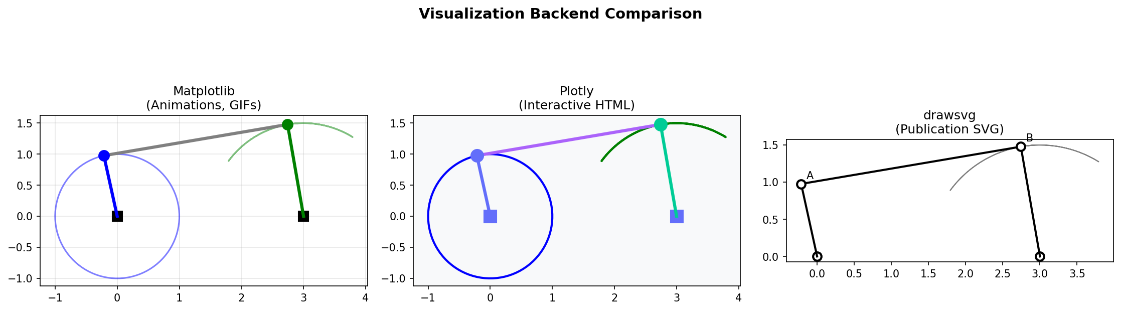
Visualization backends comparison — Comparison of the three visualization backends: Matplotlib (animations), Plotly (interactive HTML), and drawsvg (publication SVG).

Quick Reference

Backend	Best For	Output Formats
Matplotlib	Quick visualization, GIF animations	PNG, GIF, PDF, interactive window
Plotly	Interactive exploration, web embedding	HTML, PNG, PDF, SVG
drawsvg	Publications, precise vector graphics	SVG, PNG, PDF
DXF	2D CAD, laser cutting, CNC	DXF (AutoCAD compatible)
STEP	3D CAD, machining, 3D printing	STEP/STP (ISO 10303)

Matplotlib Backend

The default backend for quick visualization and animations.

Basic Visualization

import pylinkage as pl
from pylinkage.visualizer import show_linkage

# Create a four-bar linkage
crank = pl.Crank(0, 1, joint0=(0, 0), angle=0.31, distance=1, name="Crank")
output = pl.Revolute(3, 2, joint0=crank, joint1=(3, 0),
                     distance0=3, distance1=1, name="Output")
linkage = pl.Linkage(joints=(crank, output), name="Four-bar")

# Quick visualization (opens matplotlib window)
show_linkage(linkage)

Static Frame Visualization

Show the linkage at a specific position:

from pylinkage.visualizer import show_linkage
import matplotlib.pyplot as plt

# Show without animation
fig, ax = show_linkage(linkage, animated=False)

# Customize the plot
ax.set_title("Four-bar Linkage - Initial Position")
ax.grid(True, alpha=0.3)
ax.set_aspect('equal')

plt.tight_layout()
plt.savefig("linkage_static.png", dpi=150)
plt.show()

Result: A static image showing the linkage in its initial configuration.

Animated GIF Output

Create animated GIFs for documentation or presentations:

from pylinkage.visualizer import show_linkage

# Create animated GIF
show_linkage(
    linkage,
    save_path="four_bar_animation.gif",
    fps=24,                    # Frames per second
    duration=3000,             # Total duration in ms
    loci=True,                 # Show joint paths
)

print("Animation saved to four_bar_animation.gif")

Result: An animated GIF showing the linkage cycling through its motion.

Customizing Appearance

from pylinkage.visualizer import show_linkage
import matplotlib.pyplot as plt

fig, ax = show_linkage(
    linkage,
    # Display options
    loci=True,                 # Show joint trajectories
    show_legend=True,          # Add legend
    title="Custom Four-bar",

    # Style options
    joint_color='#E63946',     # Joint marker color
    link_color='#1D3557',      # Link line color
    locus_color='#A8DADC',     # Trajectory line color
    joint_size=80,             # Marker size

    # Animation options (if animated=True)
    animated=True,
    interval=50,               # ms between frames
)

plt.show()

Showing Multiple Linkages

Compare different configurations:

import pylinkage as pl
from pylinkage.visualizer import show_linkage
import matplotlib.pyplot as plt

# Create two different four-bars
def make_fourbar(d0, d1, name):
    crank = pl.Crank(0, 1, joint0=(0, 0), angle=0.31, distance=1)
    output = pl.Revolute(3, 2, joint0=crank, joint1=(3, 0),
                         distance0=d0, distance1=d1)
    return pl.Linkage(joints=(crank, output), name=name)

linkage1 = make_fourbar(3, 1, "Short rocker")
linkage2 = make_fourbar(3, 2, "Long rocker")

# Plot side by side
fig, (ax1, ax2) = plt.subplots(1, 2, figsize=(12, 5))

show_linkage(linkage1, ax=ax1, animated=False, loci=True)
ax1.set_title(linkage1.name)

show_linkage(linkage2, ax=ax2, animated=False, loci=True)
ax2.set_title(linkage2.name)

plt.tight_layout()
plt.savefig("comparison.png", dpi=150)
plt.show()

Plotly Backend

Interactive HTML visualizations ideal for web embedding and exploration.

Basic Interactive Plot

import pylinkage as pl
from pylinkage.visualizer import plot_linkage_plotly

# Create linkage
crank = pl.Crank(0, 1, joint0=(0, 0), angle=0.31, distance=1, name="Crank")
output = pl.Revolute(3, 2, joint0=crank, joint1=(3, 0),
                     distance0=3, distance1=1, name="Output")
linkage = pl.Linkage(joints=(crank, output), name="Four-bar")

# Create interactive plot
fig = plot_linkage_plotly(linkage)

# Display in notebook or browser
fig.show()

# Save to HTML
fig.write_html("interactive_linkage.html")

Result: An interactive HTML page where you can:

Zoom and pan
Hover over joints for coordinates
Toggle visibility of elements
Rotate through animation frames

Animation with Slider

from pylinkage.visualizer import plot_linkage_plotly

fig = plot_linkage_plotly(
    linkage,
    show_loci=True,            # Show joint trajectories
    show_slider=True,          # Add frame slider
    frame_count=50,            # Number of animation frames
    title="Interactive Four-bar",
)

fig.write_html("animated_linkage.html")

Result: HTML with a slider to scrub through the animation manually.

Customizing Plotly Appearance

from pylinkage.visualizer import plot_linkage_plotly
import plotly.graph_objects as go

fig = plot_linkage_plotly(
    linkage,
    # Colors
    joint_color='red',
    link_color='blue',
    locus_color='rgba(0, 255, 0, 0.5)',

    # Sizes
    joint_size=15,
    link_width=4,

    # Layout
    title="Styled Four-bar",
    width=800,
    height=600,
)

# Further customization using plotly API
fig.update_layout(
    plot_bgcolor='white',
    paper_bgcolor='white',
    font=dict(family="Arial", size=14),
)
fig.update_xaxes(showgrid=True, gridwidth=1, gridcolor='lightgray')
fig.update_yaxes(showgrid=True, gridwidth=1, gridcolor='lightgray')

fig.show()

Embedding in Web Pages

from pylinkage.visualizer import plot_linkage_plotly

fig = plot_linkage_plotly(linkage, show_loci=True)

# Get HTML div for embedding
div_html = fig.to_html(include_plotlyjs='cdn', full_html=False)

# Write to file with custom wrapper
full_html = f"""
<!DOCTYPE html>
<html>
<head>
    <title>My Linkage</title>
    <style>
        body {{ font-family: Arial; max-width: 800px; margin: auto; }}
        h1 {{ text-align: center; }}
    </style>
</head>
<body>
    <h1>Four-bar Linkage Analysis</h1>
    {div_html}
    <p>Use the controls to explore the mechanism.</p>
</body>
</html>
"""

with open("embedded_linkage.html", "w") as f:
    f.write(full_html)

drawsvg Backend

Publication-quality vector graphics for papers and documentation.

Basic SVG Output

import pylinkage as pl
from pylinkage.visualizer import save_linkage_svg

# Create linkage
crank = pl.Crank(0, 1, joint0=(0, 0), angle=0.31, distance=1, name="Crank")
output = pl.Revolute(3, 2, joint0=crank, joint1=(3, 0),
                     distance0=3, distance1=1, name="Output")
linkage = pl.Linkage(joints=(crank, output), name="Four-bar")

# Save as SVG
save_linkage_svg(linkage, "linkage.svg")

Result: A crisp SVG file that scales perfectly at any resolution.

Customizing SVG Style

from pylinkage.visualizer import save_linkage_svg

save_linkage_svg(
    linkage,
    "styled_linkage.svg",

    # Dimensions
    width=400,
    height=300,
    margin=20,

    # Colors (CSS color strings)
    joint_color='#2E86AB',
    link_color='#A23B72',
    ground_color='#F18F01',
    locus_color='#C73E1D',

    # Stroke widths
    link_width=3,
    locus_width=1.5,

    # Joint markers
    joint_radius=8,

    # Show elements
    show_loci=True,
    show_labels=True,
    show_ground=True,
)

Multi-Frame SVG

Show multiple positions in one image:

from pylinkage.visualizer import save_linkage_svg_multiframe
import pylinkage as pl

crank = pl.Crank(0, 1, joint0=(0, 0), angle=0.31, distance=1)
output = pl.Revolute(3, 2, joint0=crank, joint1=(3, 0), distance0=3, distance1=1)
linkage = pl.Linkage(joints=(crank, output))

# Show 5 evenly spaced positions
save_linkage_svg_multiframe(
    linkage,
    "multiframe.svg",
    num_frames=5,
    frame_opacity=0.3,        # Transparency of intermediate frames
    highlight_first=True,     # Make first frame solid
    highlight_last=True,      # Make last frame solid
)

Result: SVG showing the linkage at multiple positions, ideal for illustrating motion.

SVG for LaTeX

Generate SVGs optimized for LaTeX documents:

from pylinkage.visualizer import save_linkage_svg

save_linkage_svg(
    linkage,
    "latex_figure.svg",
    width=300,                 # Points (LaTeX-friendly)
    height=200,
    font_family="serif",       # Match LaTeX fonts
    font_size=10,
    show_labels=True,
    label_offset=12,
)

# Include in LaTeX:
# \begin{figure}
#     \centering
#     \includesvg{latex_figure}
#     \caption{Four-bar linkage mechanism}
# \end{figure}

CAD Export

Export linkages to industry-standard CAD formats for fabrication and 3D modeling.

Note

CAD export requires optional dependencies. Install with:

pip install pylinkage[cad]

This installs ezdxf (for DXF) and build123d (for STEP).

DXF Export (2D CAD)

Export to DXF format for AutoCAD, CNC machines, and laser cutters:

import pylinkage as pl
from pylinkage.visualizer import save_linkage_dxf, plot_linkage_dxf

# Create linkage
crank = pl.Crank(0, 1, joint0=(0, 0), angle=0.31, distance=1, name="Crank")
output = pl.Revolute(3, 2, joint0=crank, joint1=(3, 0),
                     distance0=3, distance1=1, name="Output")
linkage = pl.Linkage(joints=(crank, output), name="Four-bar")

# Save to DXF file
save_linkage_dxf(linkage, "linkage.dxf")

# Or get the ezdxf Drawing object for further customization
doc = plot_linkage_dxf(linkage)
doc.saveas("custom_linkage.dxf")

DXF Layers: The exported DXF contains organized layers:

LINKS - Link bar geometry (white)
JOINTS - Joint symbols (red)
GROUND - Ground/fixed support symbols (gray)
CRANKS - Crank/motor symbols (green)

Customizing DXF Output

Control dimensions and export a specific frame:

from pylinkage.visualizer import save_linkage_dxf

# Run simulation to get all positions
loci = list(linkage.step())

# Export frame 25 with custom dimensions
save_linkage_dxf(
    linkage,
    "frame25.dxf",
    loci=loci,
    frame_index=25,          # Export this frame (0 = first)
    link_width=0.5,          # Link bar width in world units
    joint_radius=0.2,        # Joint symbol radius
)

STEP Export (3D CAD)

Export to STEP format for 3D CAD applications (FreeCAD, SolidWorks, Fusion 360):

import pylinkage as pl
from pylinkage.visualizer import save_linkage_step, build_linkage_3d

# Create linkage
crank = pl.Crank(0, 1, joint0=(0, 0), angle=0.31, distance=1, name="Crank")
output = pl.Revolute(3, 2, joint0=crank, joint1=(3, 0),
                     distance0=3, distance1=1, name="Output")
linkage = pl.Linkage(joints=(crank, output), name="Four-bar")

# Save to STEP file (dimensions auto-scaled to fit linkage)
save_linkage_step(linkage, "linkage.step")

# Or get the build123d Compound for further manipulation
model = build_linkage_3d(linkage)
model.export_step("custom_linkage.step")

3D Geometry: The STEP export creates:

Stadium-shaped link bars (rounded rectangles extruded in Z)
Holes at joint locations for pin connections
Cylindrical pins at each joint
Ground symbols for fixed supports

Customizing STEP Dimensions

Use LinkProfile and JointProfile to control 3D geometry:

from pylinkage.visualizer import (
    save_linkage_step,
    LinkProfile,
    JointProfile,
)

# Define custom link cross-section
link_profile = LinkProfile(
    width=10.0,              # Link bar width (mm or your units)
    thickness=3.0,           # Extrusion depth in Z
    fillet_radius=0.5,       # Edge rounding (0 for sharp)
)

# Define custom joint pins
joint_profile = JointProfile(
    radius=2.0,              # Pin radius
    length=5.0,              # Pin length in Z
)

# Export with custom profiles
save_linkage_step(
    linkage,
    "machined_linkage.step",
    link_profile=link_profile,
    joint_profile=joint_profile,
    frame_index=0,           # Which position to export
    include_pins=True,       # Include joint pins
)

Exporting Multiple Frames

Export different positions of the mechanism:

from pylinkage.visualizer import save_linkage_step

# Pre-compute trajectory
loci = list(linkage.step())

# Export key positions
for i, frame_idx in enumerate([0, 25, 50, 75]):
    save_linkage_step(
        linkage,
        f"linkage_position_{i}.step",
        loci=loci,
        frame_index=frame_idx,
    )
    print(f"Exported frame {frame_idx} to linkage_position_{i}.step")

CAD Export Workflow

A typical workflow from simulation to fabrication:

import pylinkage as pl
from pylinkage.visualizer import (
    show_linkage,
    save_linkage_svg,
    save_linkage_dxf,
    save_linkage_step,
    LinkProfile,
)

# 1. Design and simulate
crank = pl.Crank(0, 1, joint0=(0, 0), angle=0.31, distance=1, name="Crank")
output = pl.Revolute(3, 2, joint0=crank, joint1=(3, 0),
                     distance0=3, distance1=1, name="Output")
linkage = pl.Linkage(joints=(crank, output))
loci = list(linkage.step())

# 2. Quick visualization to verify
show_linkage(linkage, loci=loci)

# 3. Publication figure (SVG)
save_linkage_svg(linkage, "documentation/linkage.svg", show_loci=True)

# 4. 2D CAD for laser cutting (DXF)
save_linkage_dxf(linkage, "fabrication/linkage_2d.dxf", loci=loci)

# 5. 3D CAD for machining/printing (STEP)
profile = LinkProfile(width=10, thickness=3)
save_linkage_step(
    linkage,
    "fabrication/linkage_3d.step",
    loci=loci,
    link_profile=profile,
)

print("Export complete! Files ready for fabrication.")

PSO Visualization

Visualize particle swarm optimization progress:

import pylinkage as pl
from pylinkage.visualizer import (
    plot_pso_convergence,
    plot_pso_particles,
    create_pso_dashboard,
)

# Create and optimize linkage
crank = pl.Crank(0, 1, joint0=(0, 0), angle=0.31, distance=1)
output = pl.Revolute(3, 2, joint0=crank, joint1=(3, 0), distance0=3, distance1=1)
linkage = pl.Linkage(joints=(crank, output))

@pl.kinematic_minimization
def fitness(loci, **kwargs):
    output_path = [step[-1] for step in loci]
    bbox = pl.bounding_box(output_path)
    return bbox[2] - bbox[0]  # Minimize height

bounds = pl.generate_bounds(linkage.get_num_constraints())

# Run optimization with history tracking
results, history = pl.particle_swarm_optimization(
    eval_func=fitness,
    linkage=linkage,
    bounds=bounds,
    n_particles=30,
    iters=50,
    return_history=True,
)

# Plot convergence
fig = plot_pso_convergence(history)
fig.savefig("convergence.png")

# Plot particle distribution
fig = plot_pso_particles(history, iteration=25)
fig.savefig("particles_iter25.png")

# Create full dashboard
fig = create_pso_dashboard(linkage, history, results)
fig.savefig("pso_dashboard.png", dpi=150)

Visualization with Kinematics

Show velocity vectors alongside the linkage:

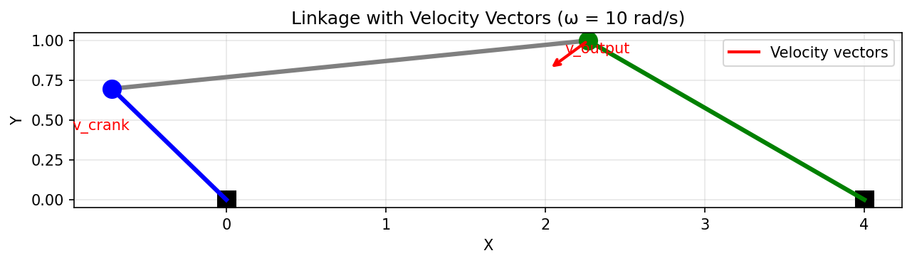
Velocity vectors visualization — Linkage with velocity vectors shown at each joint, computed from the angular velocity of the input crank.

from pylinkage.visualizer import show_kinematics, animate_kinematics
import pylinkage as pl

crank = pl.Crank(0, 1, joint0=(0, 0), angle=0.1, distance=1)
output = pl.Revolute(3, 2, joint0=crank, joint1=(3, 0), distance0=3, distance1=1)
linkage = pl.Linkage(joints=(crank, output))

# Set angular velocity
linkage.set_input_velocity(crank, omega=10.0)

# Show single frame with velocity vectors
fig = show_kinematics(
    linkage,
    frame_index=10,
    show_velocity=True,
    velocity_scale=0.05,       # Scale factor for arrow length
    velocity_color='red',
)
fig.savefig("velocities.png")

# Animated with velocities
animate_kinematics(
    linkage,
    show_velocity=True,
    save_path="velocity_animation.gif",
)

Choosing the Right Backend

Use Matplotlib when:

You need quick visualization during development
You want animated GIFs for documentation
You’re working in Jupyter notebooks
You need PDF output for simple figures

Use Plotly when:

You want interactive exploration
You’re building web applications
You need to embed in HTML pages
Users need to zoom/pan/hover

Use drawsvg when:

You’re writing academic papers
You need precise vector graphics
You want to edit the output in Inkscape/Illustrator
You need consistent styling across figures

Use DXF when:

You need to import into AutoCAD or similar 2D CAD software
You’re preparing files for laser cutting or CNC machining
You need layered 2D technical drawings
You want to edit geometry in CAD software

Use STEP when:

You need to import into 3D CAD software (FreeCAD, SolidWorks, Fusion 360)
You’re preparing files for 3D printing or machining
You want to visualize the linkage as physical parts
You need to integrate with other 3D models

Example: Complete Visualization Workflow

import pylinkage as pl
from pylinkage.visualizer import (
    show_linkage,
    plot_linkage_plotly,
    save_linkage_svg,
)

# Create an optimized linkage
crank = pl.Crank(0, 1, joint0=(0, 0), angle=0.31, distance=1, name="A")
output = pl.Revolute(3, 2, joint0=crank, joint1=(3, 0),
                     distance0=2.5, distance1=1.5, name="B")
linkage = pl.Linkage(joints=(crank, output), name="Optimized Four-bar")

# 1. Quick check with Matplotlib
show_linkage(linkage, loci=True)

# 2. Interactive exploration with Plotly
fig = plot_linkage_plotly(linkage, show_loci=True, show_slider=True)
fig.write_html("explore.html")
print("Open explore.html in browser for interactive view")

# 3. Publication figure with drawsvg
save_linkage_svg(
    linkage,
    "figure1.svg",
    width=400,
    height=300,
    show_loci=True,
    show_labels=True,
    joint_color='black',
    link_color='black',
    locus_color='gray',
)
print("Publication figure saved to figure1.svg")

# 4. Animation for presentation
show_linkage(
    linkage,
    save_path="presentation.gif",
    fps=30,
    loci=True,
)
print("Animation saved to presentation.gif")

Next Steps

Getting Started - Basic linkage creation
Kinematics-Based Optimization - Velocity visualization
See pylinkage.visualizer for complete API reference